In my earlier blog post (part 1), I posed the question of how some of the most energetic gamma-rays observed by the LHAASO and HAWC observatories can be created. In order to understand their origin, I drew an intuitive picture of how a photon can scatter off an electron at rest, usually called Compton scattering. The goal of this part is to take this a step further towards inverse Compton scattering, the case when the electron is instead moving at almost the speed of light.
Inverse Compton scattering
In all the earlier situations in part 1, the photon energy decreased or stayed the same at most. To increase the photon energy, i.e. transfer energy from the electron to the photon, the electron itself needs to have a lot of extra energy beyond its rest mass energy first! More precisely, when the electron moves very close to the speed of light, its total energy becomes dominated by the kinetic energy compared to the rest mass energy, and this kinetic energy part can then be transformed to the photon.
This inverse direction of energy transfer gives rise to the name inverse Compton scattering (although the actual scattering process is the same). To understand how suddenly energy can be transformed to the photon, we employ a common trick: We transform (also commonly called “boost”) the lab frame setup to the electron rest frame, where we know how the scattering works, and then afterwards transform back.
More specifically, in the lab frame the electron is moving very fast, but we can accelerate ourselves to be co-moving next to the electron such that in that frame the electron is at rest. We call this co-moving frame the electron rest frame. However, this transformation from one frame to the other becomes a little unintuitive, as soon as the velocity difference becomes close to the speed of light – a situation we are not used to in all-day life (see also my earlier blog post on the relativistic Christmas candle). The left two panels of Fig. 4 illustrate these relativistic transformation effects for an exemplary direction pointing upwards. In this mildly relativistic case, an electron moves at 95% of the speed of light from the top to the bottom panel. First, the originally isotropic incoming angles in the lab frame get beamed into a cone (compare the distribution of the nearly isotropic photon distribution dots on the sphere in the top panel that accumulates on the bottom in the bottom panel). Second, the original energies (green) increase in the boost direction (orange) or decrease in the opposite direction (blue). Of course, the same effects occur in the right panels, where the boost is in the other direction.
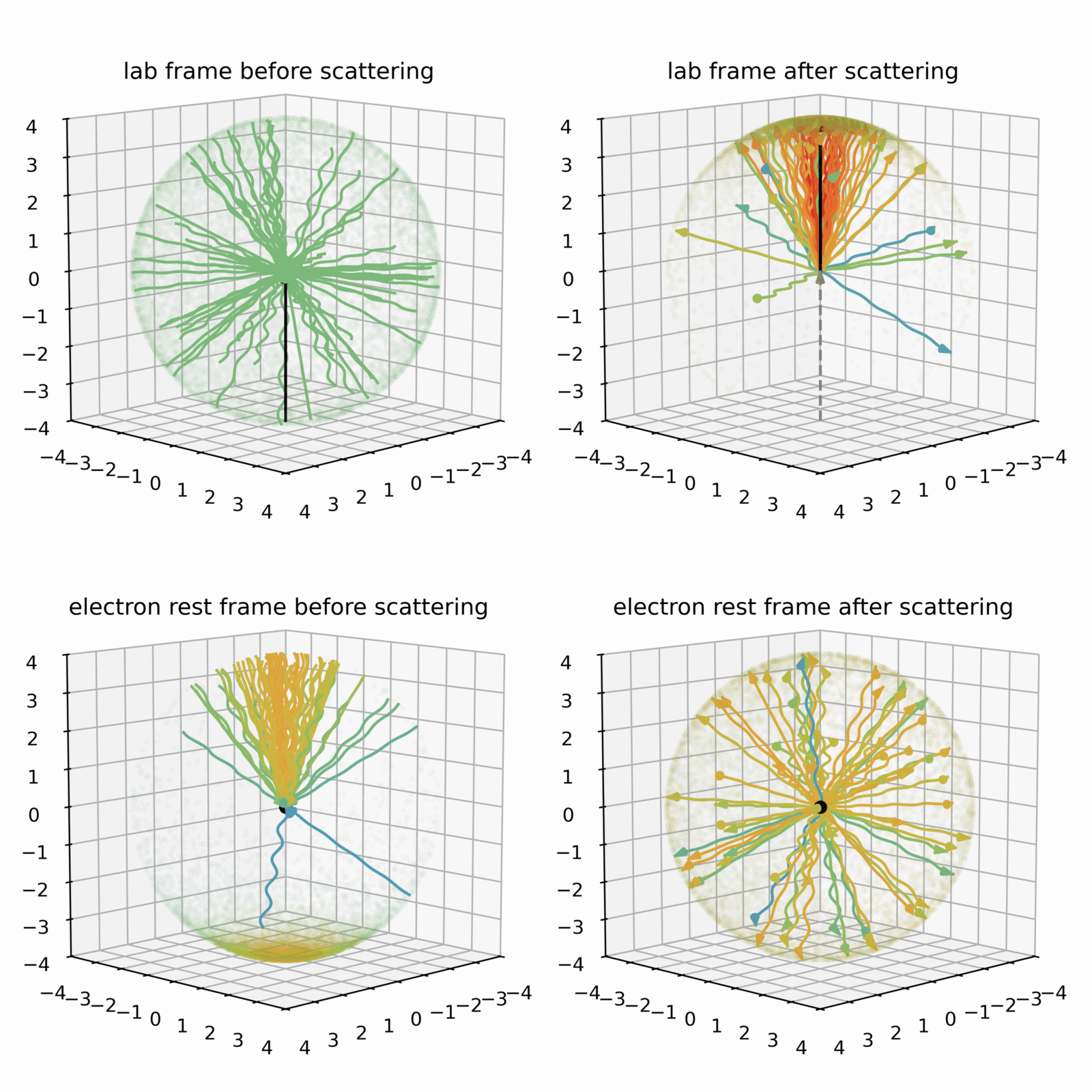
The overall logic of Fig. 4 is the following: We think of a situation where light is illuminating a volume isotropically in the lab frame and an electron is passing through with high energy (top left panel). We look at the same situation in the rest frame of the electron, where many photons of higher energy come in from a very anisotropic direction (bottom left panel). In the electron rest frame, these photons scatter following the intuition developed in part 1 of the blog and are basically isotropized again (bottom right panel) – just as in the Thomson scattering case. When we now look at that situation after scattering in the lab frame again, we do the transformation in the other direction, and photons get beamed into the cone again with an energy increase for most of them in the forward direction (top right panel). The trick we employed here is based on the fact that it doesn’t matter in which frame we are observing the physics – the same physics is going on in every frame – it is just much easier to understand in certain frames. Now when we look at the net result in the lab frame (from top left to top right panel), the electron is much more likely to scatter a photon in its forward direction and thereby increasing the photon energy. We can also observe that the electron is only minimally affected, it keeps going in the same direction and gives only a small portion of its large energy to the photon.
You might wonder now what happens, when the electron becomes more and more energetic (faster), and its kinetic energy grows orders of magnitude larger than the rest mass energy (we call this ratio the Lorentz factor)? This is the case we observe in multiple astrophysical environments, where the Lorentz factor can reach values of thousands to millions (even billions). The more energetic the electron, the faster the transformation (“the larger the boost”), so the smaller the cone in which the photons become beamed, and the larger the energy gain. This situation is illustrated in Fig. 5, which is similar to Fig. 4, but shows the stronger beaming and energy increase.
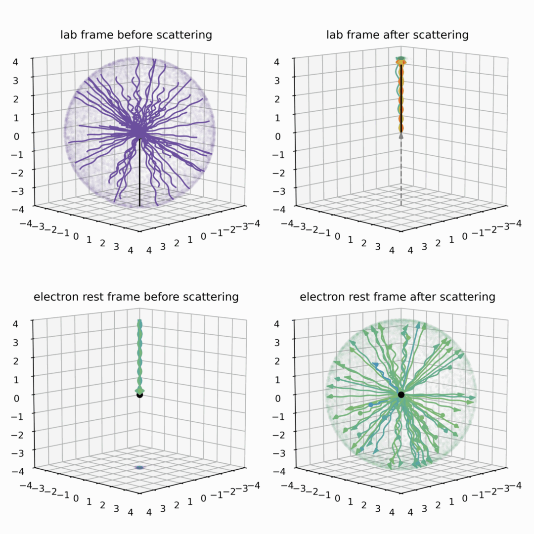
We successfully transferred a lot of energy to the photon – and we could understand that in the same framework as earlier. It is the direction change between the two large boosts that makes them add up and transfer the energy so efficiently.
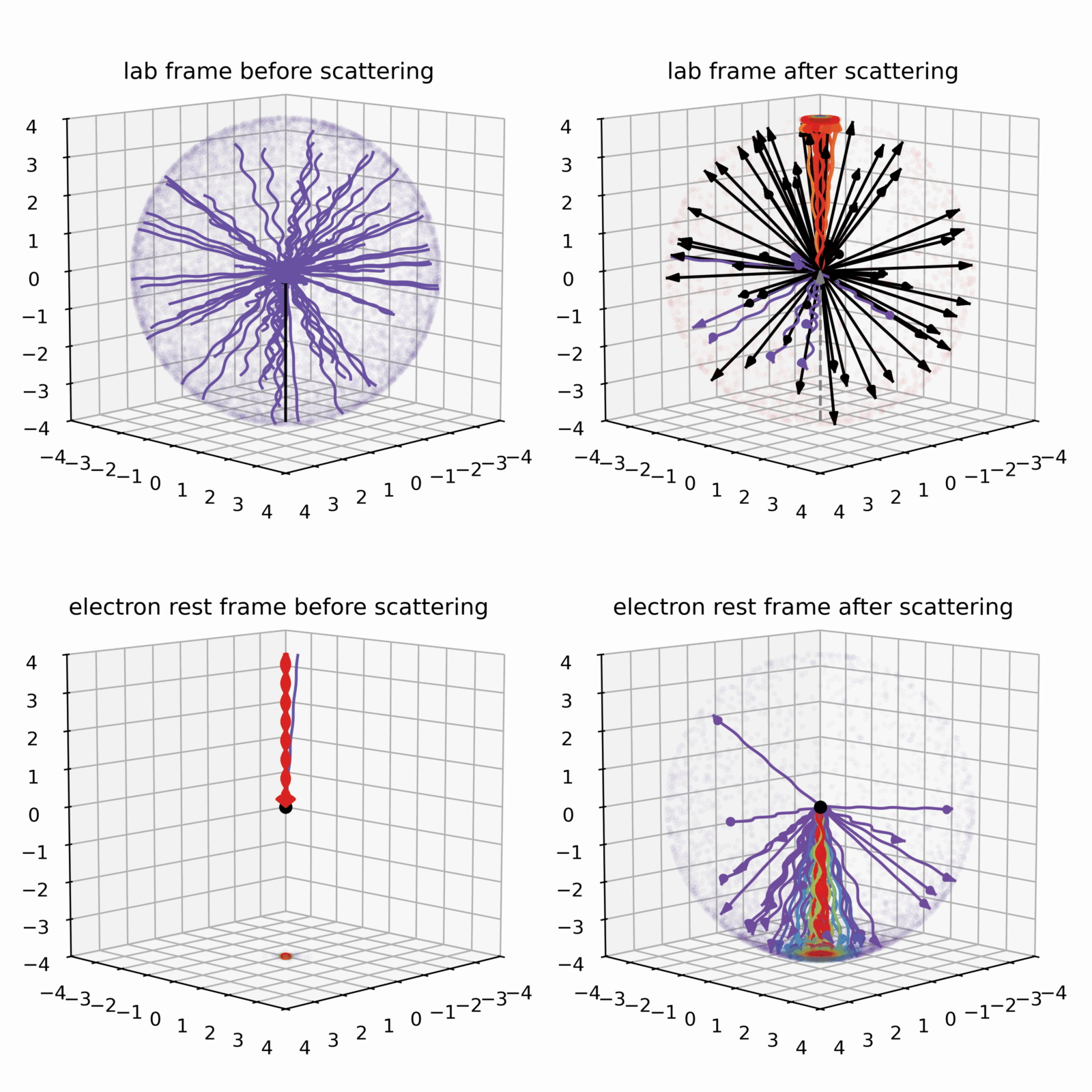
Now you might wonder what happens when the photon energies in the electron rest frame (bottom left panel) become comparable or larger than the electron rest mass? We saw earlier that then the Compton scattering gets suppressed into the forward cone – the Klein-Nishina effect. This situation is illustrated in Fig. 6, where now the scattering occurs primarily in the forward direction (bottom right panel). Nevertheless, the strong boosting transformation beams the forward beam (pointing downwards) into the electron’s direction of motion (pointing upwards), when observed in the lab frame. Additionally, something else is visible in the lab frame (upper right panel): after the scattering, the electron gets significantly deflected as well (all the black arrows, again just the direction without the magnitude). This deflection means simply that the electron transfers almost all of its extremely large energy to the photon, which is then mostly directed in the same direction as the electron before (conservation of the total momentum).
Compton scattering summary
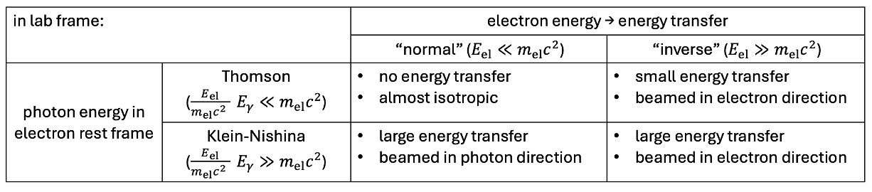
To wrap this up: Charged particles like electrons and light (photons) do interact with each other, generally called Compton scattering. The nature of the interaction depends on the electron energy that determines the direction of the energy transfer (normal vs inverse), and on the photon energy as measured in the electron rest frame, that determines whether scattering happens in the Thomson or Klein-Nishina regime. The different combinations are summarized in the table below:
Origin of the astrophysical ultra-high-energy photons
As we saw, inverse Compton scattering can be an efficient process to transfer large amounts of energy from very fast electrons to photons. Obviously, both high-energy electrons and low energy target photons need to be present in the astrophysical system for that. The existence of low energy photons is often easier to test, as they typically freely stream around and escape the system and shine towards us. We can “just” observe the system and see what target photons there are available. In contrast, the high-energy electrons are typically expected to be deflected by magnetic fields all the time, effectively confining them to the source region for a long time. And even if they escape, the turbulent magnetic fields on their way deflect them into all directions, making it impossible to “just observe the system with an electron camera”. Thus, we instead study these energetic electrons indirectly, by detecting the gamma rays that they create via inverse Compton scattering. These are exactly the gamma rays that LHAASO and HAWC observed, which in turn allows us to infer exciting information about the local environment, i.e. how the electrons are being accelerated and how they interact with other components like the local magnetic fields. It is therefore only the fundamental bouncing interaction between light and electrons that makes it possible to learn more about the distant mysteries of some of the extremest spots of the universe.
The code to generate these plots can be found here.
")

