As introduced in the previous posts, nowadays it is well known that spacetime is not always ‘flat’ but can be distorted by the presence of massive (dense) objects, according to Albert Einstein’s general theory of relativity. The amount of distortion in spacetime depends on the mass of the object and on how compact it is. Prof. John Wheeler, a theoretical physicist in the US, told that “Spacetime tells matter how to move; matter tells spacetime how to curve“. According to Einstein’s theory, light always follows the shortest path through spacetime, implying that the light paths are no longer straight lines but can be curved in the immediate vicinity of massive and compact objects, e.g., black holes.
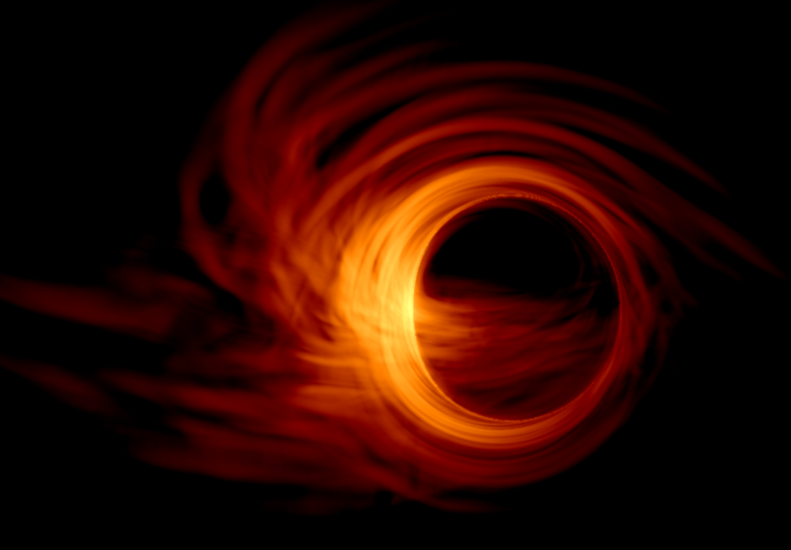
While our understanding of the curved spacetime around the compact objects has been significantly improved over decades, the question was what it would look like near the black hole. There have been many theoretical models to infer the image around the black hole, and many people could enjoy the cinematic visual of the black hole from the movie “Interstellar” which was advised by the scientific modeling. In 2019, the question was finally answered by the Event Horizon Telescope (EHT) collaboration, which delivered the first image of a black hole, revealing a bright “photon ring” and a “black hole shadow”.
Then other key questions follow as to what is going on around the black hole, how we can interpret this observed image, and which information we can obtain from it. To answer these questions, astrophysicists make use of either semi-analytic modeling or numerical simulations. The major difference between them is while the semi-analytic models assume that the flows are in a steady state (no variation in time), the numerical simulations let the flows evolve from the initial model under the conservation laws. Those are complementary to each other since the numerical simulations are computationally way more expensive than the semi-analytic approach.
We have an observed image of the black hole and numerical datasets that depict the flow motions around it. What is next? Of course, most importantly we have to evaluate the numerical results if they are in good agreement with the observation. Since the simulations print out only the timely evolved physical properties of the fluids such as mass density, energy density, velocity, magnetic fields, not the radiative properties, the post-process should be conducted to calculate the light images from the numerical dataset. For this case, what we can use is the general-relativistic radiative transfer (GRRT) codes, which have been developed independently from many groups, e.g., BHOSS, GRmonty, iPole, Raptor. You may consider these GRRT tools as a bridge between numerical datasets and observed images (or spectra).
These GRRT tools employ the basic idea that electromagnetic radiation (light) is described by null geodesics of the background spacetime, which is integrated backward in time from the observer, called “ray-tracing”. The radiation running backwards would end up with (1) escaping to infinity, (2) being captured by the black hole, or (3) being absorbed by the accretion flow: Since the black holes are gravitational intense, if a passing photon is a bit too close, it will be trapped on orbit around the black hole, yielding a bright “photon ring” (see movie 1).
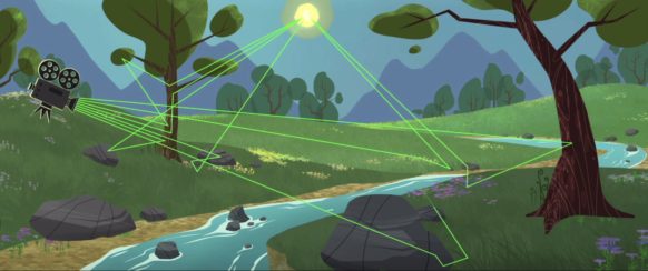
The ray-tracing in GRRT tools is somewhat akin to the light paths that the modern 3D animation movies have adopted (see Figure 1 and the link for Disney’s guide). Similarly, in the 3D animations, if the scene has a light source (like the Sun in the Figure), the camera collects all the lights that have been scattered and reflected on their way from the source. In GRRT calculation, all radiative processes including absorption and emission (and/or scattering) are being computed through the path of the photon. However, as you might already notice, there has never been the gravitationally intense object in the Pixar or Dreamwork 3D animations (if there are, I apology :)), which bends the light path. So the light path in the animation would be always straight, which is obviously different from GRRT calculation!
As a member of the EHT collaboration, our group has devoted to understand the dynamical evolution around the black holes for both observational and theoretical perspectives (as an example, see movie 2 below which shows the simulated fluid properties and the post-processed radiative properties). I recall what one professor told in the fundamental astronomy class when I was a college student that “astronomy is very beautiful because it is one of a few academic fields that can improve our knowledge by communicating actively between theorists and experimentalists (here observational astronomers)”.